Back in January of 2017 (yes, this blog has a large and distinguished backlog), we went to an art exhibition at The Dixon here in Memphis, TN. It was the debut of a special exhibition organized by The Crystal Bridges Museum in Arkansas. There was a great little write-up in a local, independent paper.
And when I say great, I mean both that it was well-written and that it mentioned two of my favorite pieces in the exhibition. To be fair, there were a LOT of pieces that I found clever, funny, moving, wow-inducing, and often a mixture of all of those.
However, one piece in particular jumped out at me: End of the Spectrum by “Ghost of a Dream”. Ghost of a Dream is a collaboration of the artists Lauren Was and Adam Eckstrom. I haven’t placed an image of the piece here out of respect for the artists, but you can see an image at their website under the More Collages section.
As most savvy readers have guessed by now, it’s a collage. What you might not know (unless you cheated) is that Was and Eckstrom created the collage using nothing but lottery tickets. Since this is the blog of a math/data/tech nerd, you probably know where this going…
You aren’t going to win the lottery
How do I know that? Well, I don’t, but I’m pretty damn certain. How certain? Let’s do some math. Actually, let’s not. There are plenty of mathy explanations about lotteries and winning and what not out there. (There’s a complete but dense read over at Wikipedia.)
Instead, let’s actually use our computers for something besides reading blogs.
In fact, I believe one enormous advantage we ultra-modern geeks have over the nerds of yore is the ability to quickly simulate models with a computer. And I’m not talking about freely available software packages to simulate complicated fluid dynamics over rigid objects, although those exist! No, I’m talking about starting with some simple assumptions and working out some consequences.
So how do we do that? To start with we do some googling to find out the odds of winning the Powerball. We’ll go with 1 chance to 292 million. From there we can cobble together a function to keep simulating a lottery draw until we win in Python:
from scipy import rand

def one_chance():
    CHANCE = 1.0 / (292000000.0)
    count = 0
    while True:
        count += 1
        if rand() <= CHANCE:
            return count
So every time we call one_chance, we get a single simulated answer: how many
lottery tickets we bought before we won the Powerball. The problem is that this
is one single, solitary simulation. How do we know if we’re close? Without
doing any math, we need to simulate a lot. To start, how about we just simulate
10,000 wins? Uh, don’t do that. On my reasonable-ish computer the above
simulation spit out 414,883,780 after about 5 minutes. 10,000 times 5 minutes
is almost 2 weeks.
Now sure, there are ways to speed up our simulation, and there also ways to use multiple cores. But we violated one of the cardinal rules of simulation before we started… Namely, do all the analytical work you can up front. Sadly for you, dear reader, that’s means doing math. Luckily for you, though, I tend to use a slightly different rule. I do analytical work until I get annoyed, and then I start coding. Well, not always, but in this case yes.
In this case, let’s think about what we really want to know. I’m going to reframe “How many times do I need to buy a lottery ticket” as “If I buy X lottery tickets a week, how long until I win?”. That’s tough, too. So how about, “If I know that every lottery ticket I buy increases my chances of winning, how long until I have a 50-50 shot?”
So now things are about to get a little more complicated… Let’s define \(W\) as the probability of winning the Powerball on a single draw. Recall that above we set \(W = \frac{1}{292,000,000}\). What do know about \(W\)? I mean, other than it’s teeny-tiny? Well, we know that it’s a binary variable: either we won or we didn’t. So the probability of not winning the lottery on a single draw is \(1 - W\). If this doesn’t make sense, think of it this way: probabilities are like percentages. They always add up to \(100\%\).
Let’s call \(L\) the chance of losing the lottery. So if \(W\) is 1 in 292 million, then \(L = 1 - W = 1 - \frac{1}{292,000,000} = 0.9999999965753424\). Or if you prefer, \(99.99999965753424\%\). That’s a pretty good chance at not winning the lottery.
So what are the chance that you’ll lose 3 times in a row? We’re going to assume that any two lottery tickets are independent; that is, it doesn’t matter where or when you buy them, they all have the same chance of winning. If that’s the case, then we know that multiplying two probabilities gives us the chance of them both happening. So the probability of losing 2 times in a row is \(L \times L\) and the probability of losing 3 times in a row is \(L \times L \times L = 0.9999999897260273\) or \(99.99999897260273\%\).
I’ll save your eyeballs the work of checking: that’s \(0.00000000684931511508\) lower than buying one ticket. Not much of a change, but it is a change. So we can keep multiplying \(L\) until we get to \(50\%\)!
But wait - there’s a problem. Old Experienced software engineers all
know what’s coming… the dreaded floating point lecture. The most common way
of representing numbers with decimal parts is called “floating point”. It’s so
common that pretty much every major CPU on the market comes with special
hardware for working with floating point numbers. But they aren’t perfect.
Because they have to estimate decimal numbers, multiplying lots of small
floating points together can cause you to get wrong (and in some cases strange)
answers. Ideally we would rather add numbers instead of multiply, and we would
like the numbers to be similar in size.
Which brings us to…
Logarithms
Logarithms power slide rules. If you don’t know what a slide rule is, watch Apollo 13. When the NASA math peeps grab something that looks like a ruler to do math? That’s a slide rule. Before electronic calculators or computers, engineers and other mathy folks used slide rules to handle lots of computations. How do logarithms help with that?
If you’re not familiar with logarithms, forget what you were probably told in school about exponents. That was all true, but for the moment, just think about them as a transformation. A unit conversion as it were, like converting from Fahrenheit to Celsius so that you can explain to your European friends how freaking hot is gets in Memphis. But instead you’re converting from normal numbers to easy-to-multiply numbers. Our usual numbers are easy to add, but a little more complicated to multiply.
You’re probably already used to logarithms. The pH measure as in “pH Balanced”, the dB (decibel) rating for audio, and the Richter scale for earthquakes are all numbers in these special easy-to-multiply number units. Logarithms are incredibly handy and come in different sizes. Those of us who use them refer to these sizes as the base. The most common bases are \(e\) (the natural number), 10, and 2 (a favorite for computer scientists). For all of our examples we’ll be using base \(e\). One advantage of this is that most computing environments have a function to convert from logarithms back to normal numbers: \({\exp}\) 1.
When you convert a regular numbers with logarithms, adding the new numbers is the same as multiplying the original numbers. So let’s start with the numbers \((2,3,4)\). If we multiply them all together we get \(2 \times 3 \times 4 = 24\).
If we convert these numbers to logarithms we get
\(\log(2), \log(3), \log(4) = (0.69314718, 1.09861229, 1.38629436)\)
And just like magic,
\(\exp(0.69314718 + 1.09861229 + 1.38629436) = 24\)
That’s much easier to work with, amirite! Well, it’s not for you, but it is for computers. It’s easier to see if the numbers are far apart. What about:
Those numbers are much closer to each other… and the closer they are the less error we introduce when we perform floating point operations. Adding numbers that are close together is much, much better than multiplying lots of tiny numbers that get progressively tinier (or larger). Now that we have that trick under our belt, we can actually do some calculating.
import scipy as sp

def keep_buying():
    MILLION = 1000000.0
    CHANCE = 1.0 / (292 * MILLION)
    LOSER = 1.0 - CHANCE

    LOG_LOSER = sp.log(LOSER)

    TICKETS_BOUGHT = 5000
    curr = LOG_LOSER
    count = 0

    while sp.exp(curr) > 0.50:
        count += TICKETS_BOUGHT
        curr += (LOG_LOSER * TICKETS_BOUGHT)

    return count, sp.exp(curr)
You’ll note that instead of evaluating every single purchase of a lottery
ticket, we increment by TICKETS_BOUGHT. You can play around with that
parameter: smaller numbers will make our tiny function run longer but give us
more accurate answers.
If Only Socrates Hadn’t Drank That
I’ll save you the suspense: our function returns \((202400000, 0.4999982431545981)\).
That’s a lot of tickets! \(\frac{202400000}{365.25} \approx 554141\), so purchasing one ticket a day for 554 thousand years will get us a \(50\%\) chance at winning the Powerball. That’s… a long time. So we need to buy more tickets per day. Let’s imagine that Socrates starts buying 50 Powerball tickets every, single day in 450 BCE (he would be around 19-20 years old then). His odds of winning the Powerball would hit 50% some time after 10,000 AD. And, of course, because everything is better with an xkcd-style graph…
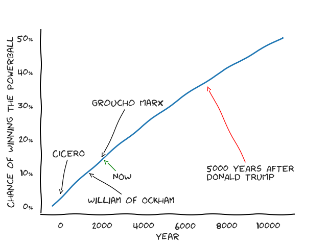
We can now state that unless you’re Socrates, immortal, have endless wealth, and want to buy lottery tickets every day for \(10,000\) years, maybe don’t play the lottery. Or do - at least in Tennessee it supports education.
References
Links used in this article (or that you might want to check out):
- Crystal Bridges Museum of American Art: http://crystalbridges.org/
- Dixon Gallery & Gardens: http://www.dixon.org/
- Ghost of a Dream: https://www.ghostofadream.com/
- Logarithms @ Wikipedia: https://en.wikipedia.org/wiki/Logarithm
- Lottery Math @ Wikipedia: https://en.wikipedia.org/wiki/Lottery_mathematics
- Memphis, TN Wikipedia Page: https://en.wikipedia.org/wiki/Memphis,_Tennessee
- More Collages from Ghost of a Dream: https://www.ghostofadream.com/more-collage
- Powerball @ Wikipedia: https://en.wikipedia.org/wiki/Powerball
- Slide Rules: https://en.wikipedia.org/wiki/Slide_rule
- Socrates @ Stanford Encyclopedia of Philosophy: https://plato.stanford.edu/entries/socrates/
- ‘State of the Art’ at the Dixon: http://www.memphisflyer.com/memphis/state-of-the-art-at-the-dixon/Content?oid=5203984
- The Memphis Summer Bucket List: https://choose901.com/memphis-summer-bucket-list/